Exercises
We have seen that it could be extremely beneficial to compute \(C=A\times B^T\) by directly implementing a mult_trans operation rather than explicitly forming the transpose of \(B\) and calling mult.
In this exercise we are going to explore a few more details about optimization.
mult vs. mult_trans
Your starter repository contains a benchmark driver mmult.cpp that exercises the matrix multiply and matrix multiply transpose operations we wrote in the last assignment. It loops over a set of matrix sizes (8 to 256) and measures the performance of each function at that size. For each size it prints a row of performance numbers in GFlop/s – each column is the performance for one of the functions.
The functions mult_0 through mult_3 and mult_trans_0 through mult_trans_3 are provided for you. Compile and run mmult (the default size used with no command line argument should be fine). There is a rule in the provided CMakeLists.txt that invokes the compiler so you should just be able to build the program and run it afterwards:
$ ./build/mmult
Please make sure to compile all tests related to measuring performance in
Releasemode.
If your computer and compiler are more or less like mine, you should see something printed that looks like this:
  N      mult_0      mult_1      mult_2      mult_3     mul_t_0     mul_t_1     mul_t_2     mul_t_3
  8     3.00795     2.90768     6.23075     5.81536      3.6346     3.35502     7.93004     7.26921
 16     2.35758      2.4572     6.23075     6.12144     2.50123     6.58343     11.0769     11.8279
 32     1.98706     2.01804     6.61387     6.56595     2.29975     12.0813     15.8965      17.425
 64     1.70172     1.94222     6.08737     6.62057     2.05673     13.9541      20.156     17.7847
128     1.57708     1.72746     6.05582     6.35951     1.79506     14.7662      21.136      16.457
256     1.28681     1.46371     4.87796     5.92137     1.62958      11.073     19.4263     15.7063
Huh. Although we applied all of the same optimizations to the mult and mult_trans functions – the mult_trans functions are significantly faster – even for the very simplest cases. That is fine, when you need to compute \(C = A\times B^T\) – but we also need to just be able to compute \(C = A\times B\) – it is a much more common operation – and we would like to do it just as fast as for \(C = A\times B^T\).
- Save the output from a run of
mmultinto a fileresults/mmult.logand submit that as part of your homework.
Loop Ordering
The mathematical formula for matrix-matrix product is
\[C_{ij} = \sum_{k=0}^{K-1} A_{ik} B_{kj} ,\]which we realized using our Matrix class as three nested loops over i, j, and k (in that nesting order). This expression says “for each \(i\) and \(j\), sum each of the \(A_{ik} B_{kj}\) products.
The function(s) we have been presenting, we have been using the “ijk” ordering, where i is the loop variable for the outer loop, j is the loop variable for the middle loop, and k is the loop variable for the inner loop:
void mult(const Matrix& A, const Matrix& B, Matrix& C)
{
    for (size_t i = 0; i < C.num_rows(); ++i)
        for (size_t j = 0; j < C.num_cols(); ++j)
            for (size_t k = 0; k < A.num_cols(); ++k)
                C(i, j) += A(i, k) * B(k, j);
}
But the summation is valid regardless of the order in which we add the k-indexed terms to form each result matrix element $C_{ij}$$. Computationally, if we look at the inner term C(i, j) = C(i, j) + A(i, k) * B(k, j) – there is no dependence of i on j or k (nor any of the loop indices on any of the other loop indices); we can do the inner summation in any order. That is, we can nest the i, j, k loops in any order, giving us six variants of the matrix-matrix product algorithm. For instance, an “ikj” ordering would have i in the outer loop, k in the middle loop, and j in the inner loop.
void mult_ikj(const Matrix& A, const Matrix& B, Matrix& C)
{
    for (size_t i = 0; i < C.num_rows(); ++i)
        for (size_t k = 0; k < A.num_cols(); ++k)
            for (size_t j = 0; j < C.num_cols(); ++j)
                C(i, j) += A(i, k) * B(k, j);
}
Benchmark Different Loop Orderings
The program mmult_indices.cpp in your work directory is a benchmark driver that calls six different matrix multiply functions: mult_ijk, mult_ikj, mult_jik, mult_jki, mult_kij, and mult_kji. The corresponding implementations are included in your matrix_operations.cpp file. Right now those implementations are completely unoptimized – they are each just three loops (in the indicated order, with C(i, j) += A(i, k) * B(k, j) in the inner loop). The program runs each of these six functions over a set of problem sizes (\(N \times N\) matrices) from 8 to 256, in powers of two. The maximum problem size can also be passed in on the command line as an argument. The program prints the GFlop/s that it measures for each of the six functions, for each of the sizes it runs.
Compile and run mmult_indices (the default arguments should be fine). There is a CMake rule that builds this executable. Please make sure to build in Release mode (as usual for performance measurements):
$ ./build/mmult_indices
Look carefully at the performance numbers that are printed. You should see two of the columns with not so good performance, two columns with okay performance, and two columns with the best performance. The columns within each pair have something in common – what is it?
Depending on your CPU and your compiler, some of the differences will be more or less pronounced, but they should be visible as the problem size increases.
Here is a discussion question for you on Discord. Explain what you are seeing in terms of data accesses at each inner loop iteration.
Save the output from a run of mmult_indices with “_0” in the results folder (i.e. as results/mmult_indices_0.log) to indicate it is a run before any optimizations have been introduced.
Answer the following questions in
results/answers.md:
- There are three pairs of index orderings that give similar performance. What have those orderings in common?
- Save the output from a run of
mmult_indicesinto a fileresults/mmult_indices_0.logand submit that as part of your homework.
What is the Best Loop Ordering?
I claim that certain loop ordering give good performance because of the memory access pattern being favorable. Is that consistent with what you are seeing in these (unoptimized) functions?
To guide your discussion, consider the following diagram of matrices A, B, and C.
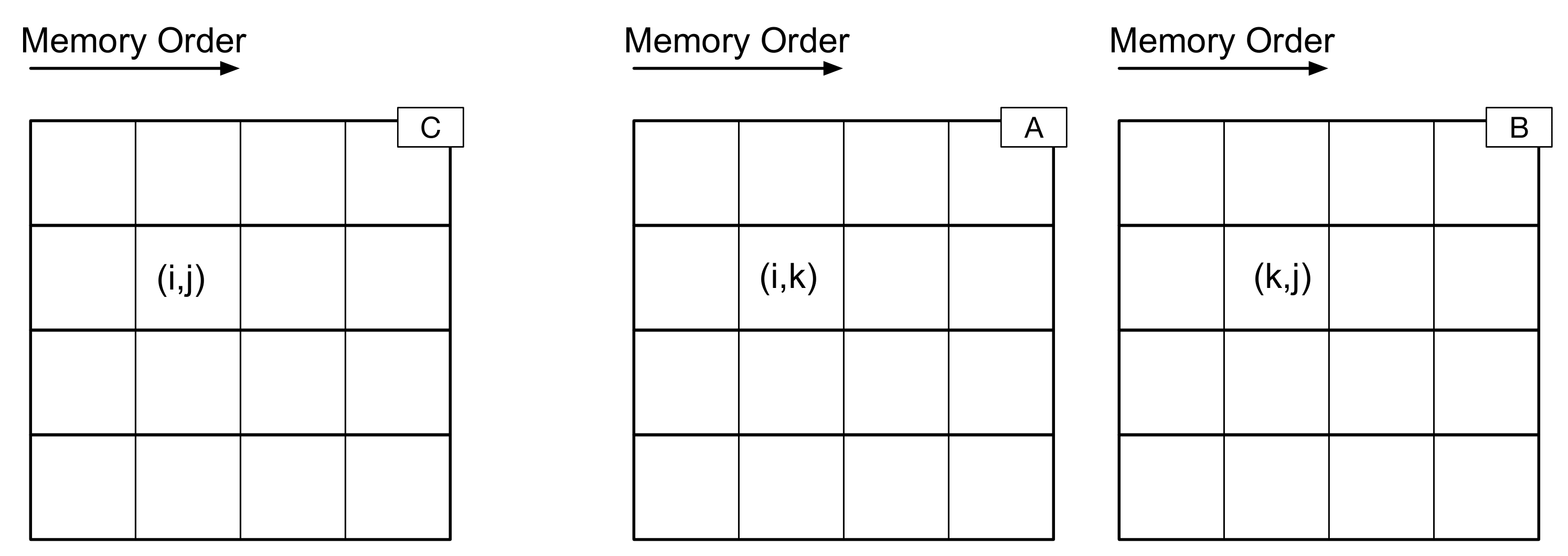
Here, each box is a matrix entry. Recall that for row-ordered matrices (such as we are using in this course), the elements in each row are stored next to each other in memory.
Now, let’s think about what happens when we are executing matrix multiply with the “ijk” ordering. From one iteration of the inner loop to the next (from one step of the algorithm to the next), what are the next data elements to be accessed? For “ijk”, here is what happens next:
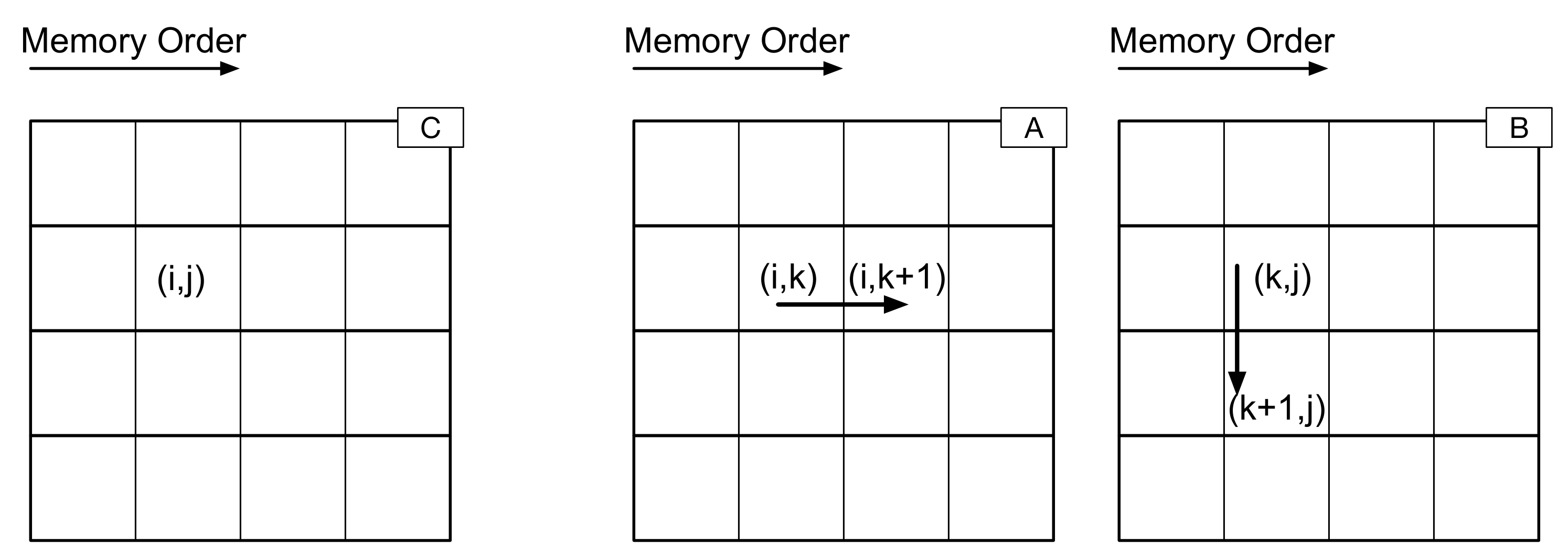
What happens in the case of each of the six orderings for mult – what are the next elements to be accessed in each case? Does this help explain the similarities between certain orderings – as well as why there are good, bad, and ugly (er, medium) pairs? Refer again to how data are stored for three matrices A, B, and C.
Answer the following question in
results/answers.md:
- Referring to the figures about how data are stored in memory, what is it about the best performing pair of loops that is so advantageous?
Optimizing mult_trans
If we look at the output from mmult, the biggest jump in performance comes between mult_trans_0 and mult_trans_1. The difference between the code in the two functions is quite small though – we just “hoisted” the reference to C(i, j) out of the inner loop.
What will the data access pattern be when we are executing mult_trans in “ijk” order? What data are accessed in each of the matrices at step (i, j, k) and what data are accessed at step (i, j, k+1)? Are these accesses advantageous in any way?
Answer the following questions in
results/answers.md:
- Referring again to how data are stored in memory, explain why hoisting
C(i, j)out of the inner loop is so beneficial inmult_transwith the “ijk” loop ordering.
Using mult_trans to Optimize mult (Take 1)
Modify mult_ijk so that it achieves performance on par with mult_trans_1 (or mult_trans_2 or mult_trans_3). (Hint: Be lazy: mult_trans_1 et.al. are already written. Don’t repeat yourself. Don’t even copy and paste.)
Compile and run mmult_indices with your modified version of mult_ijk. Save the output to a file results/mmult_indices_1.log.
Sometimes when you are developing code, you might want to keep older code around to refer to, or to go back to if an exploration you are making doesn’t pan out. One common way of saving things in this way is to use the preprocessor and “#if 0” the code you don’t want to be compiled.
#if 0
Stuff I want to save but not compile
#endif
You may (but are not required) to “#if 0” the initial version of mult_ijk.
Answer the following questions in
results/answers.md:
- Save the output from a run of your optimized
mmult_indicesinto a fileresults/mmult_indices_1.logand submit that as part of your homework.
Using mult_trans to Optimize mult (Take 2)
Modify mult_3 so that it achieves performance on par with trans_mult_1 (or trans_mult_2 or trans_mult_3). (This may not be quite as straightforward as for mult_ijk).
Compile and run mmult_indices with your modified version of mult_3 with problem sizes up to 1024 (say). Save the output to a file results/mmult_indices_2.log.
Answer the following question in
results/answers.md:
- What optimization is applied in going from
mult_2tomult_3?- How does your maximum achieved performance for
mmult_indices(any version) compare to whatbandwidthandrooflinepredicted? Show your analysis.- Save the output from a run of your optimized
mmult_indicesinto a fileresults/mmult_indices_2.logand submit that as part of your homework.
Array of Structs vs. Struct of Arrays
To store the “color” of a particular pixel, a color image stores the values of the three additive primary colors (red, green, and blue) necessary to reconstruct that color. A color image is thus a three-dimensional structure: 3 color planes, each of which is the same height by width of the image.
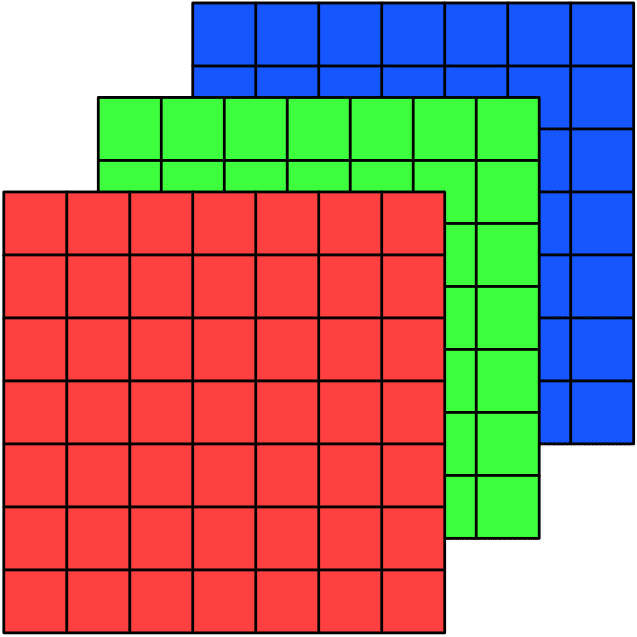
A question arises then about what is the best way to store / access that data in memory? We could, for instance, store each color plane separately, so that the image is a “structure of arrays”:
![]()
Or, we could store the three color values of each pixel together, so that the image is an “array of structures”:
![]()
Or, we could store just a single large array, treating the image as a “tensor” and use a lookup formula to determine how the data are stored.
The struct of arrays data structure could be implemented like this:
class SOA_Image {
public:
    SOA_Image(size_t M, size_t N)
      : nrows(M)
      , ncols(N)
      , storage
    {}

    size_t num_rows() const { return nrows; }
    size_t num_cols() const { return ncols; }

    const double& operator()(size_t i, size_t j, size_t k) const {
        return storage[k][i * ncols + j];
    }
    double&       operator()(size_t i, size_t j, size_t k) {
        return storage[k][i * ncols + j];
    }

private:
    size_t                             nrows;
    size_t                             ncols;
    std::array<std::vector<double>, 3> storage;
};
Again, the terminology “struct of arrays” is generic, referring to how data are organized in memory. Our implementation (in storage) of the “struct of arrays” is as a array of vector. Note also that the accessor operator() accesses pixels with (i, j, k) where i and j are pixel coordinates and k is the color plane.
Similarly, the array of structs data structure could be implemented this way:
class AOS_Image {
public:
    AOS_Image(size_t M, size_t N)
      : nrows(M)
      , ncols(N)
      , storage(M * N)
    {}

    const double& operator()(size_t i, size_t j, size_t k) const {
        return storage[i * ncols + j][k];
    }
    double&       operator()(size_t i, size_t j, size_t k) {
        return storage[i * ncols + j][k];
    }

    size_t num_rows() const { return nrows; }
    size_t num_cols() const { return ncols; }

private:
    size_t                             nrows;
    size_t                             ncols;
    std::vector<std::array<double, 3>> storage;
};
Again, the terminology “array of structs” is generic. Our implementation (in storage_) of the
“array of structs” is as a vector of array. Note also that the accessor operator() accesses pixels with (i, j, k) where i and j are pixel coordinates and k is the color plane.
Finally, a “tensor” based storage could be implemented as:
class Tensor_Image {
public:
    Tensor_Image(size_t M, size_t N)
      : nrows(M)
      , ncols(N)
      , storage(3 * M * N)
    {}

    const double& operator()(size_t i, size_t j, size_t k) const {
        return storage[k * nrows * ncols + i * ncols + j];
    }
    double&       operator()(size_t i, size_t j, size_t k) {
        return storage[k * nrows * ncols + i * ncols + j];
    }

    size_t num_rows() const { return nrows; }
    size_t num_cols() const { return ncols; }

private:
    size_t              nrows;
    size_t              ncols;
    std::vector<double> storage;
};
Blurring
Although blurring an image sounds like something you would not want to do, small amounts of blur can be useful in image processing for, say, removing high frequency noise from an image. One simple blurring function is a box blur, which computes an output pixel based on the average of nine neighboring input pixels.
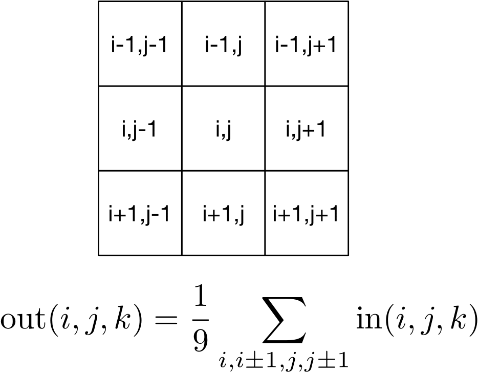
So, for instance, we could blur an image with the following:
// Iterate through the image
for (size_t i = 1; i < img.num_rows() - 1; ++i) {
    for (size_t j = 1; j < img.num_cols() - 1; ++j) {
        // Iterate through the color planes
        for (size_t k = 0; k < 3; ++k) {
            // Apply blurring kernel
            blurred(i, j, k) = (
                img(i + 0, j + 0, k) +
                img(i + 0, j + 1, k) +
                img(i + 0, j - 1, k) +
                img(i + 1, j + 0, k) +
                img(i + 1, j + 1, k) +
                img(i + 1, j - 1, k) +
                img(i - 1, j + 0, k) +
                img(i - 1, j + 1, k) +
                img(i - 1, j - 1, k)) / 9.0;
        }
    }
}
Note that since we have defined the accessor generically, the inner blurring kernel will be the same regardless of which representation we use for the image. We do have a choice, however in how we access the data: do we iterate over the color planes as the outer loop or as the inner loop?
Loop Ordering
In your source code for this assignment is the file soa_vs_aos.cpp. From it you can generate soa_vs_aos. When you run that executable on an image, it will apply six different blurring operations: for the three different formats (aos, soa, tensor) and for the image planes iterated on the outer loop and on the inner loop. Read the source code to familiarize yourself with which blurring kernel does which. Note, as mentioned above, that the inner loop of each function is the same – and that the functions doing the color plane on the outer loop are the same (similarly for the inner loop). (If it seems like we are violating DRY, we are, we will see how to fix this in a few more assignments.)
Your source code has one julia image: results/julia.bmp. You can generate your own images based on your previous assignment, however. Run the program on them. The program will print out execution times for the six implementation variants of the blurring function as well as save the blurred output for each variant. (If you don’t want to see these (or spend the time computing them), you can comment out the lines in the code that save the output images.):
$ cd results
$ ../build/soa_vs_aos julia.bmp
Answer the following questions in
results/answers.md:
- Which variant of blurring function between struct of arrays and array of structs gives the better performance? Explain what about the data layout and access pattern would result in better performance.
- Which variant of the blurring function has the best performance overall? Explain, taking into account not only the data layout and access pattern but also the accessor function.
Next up: Buddhabrot Fractal